The goal is to calculate historical returns for a leveraged S&P 500 ETF, since there is no historical data for e.g. the UPRO. The full analysis, including all code, is available as a Jupyter notebook: open the notebook (HTML).
We try to hit the UPRO (3x S&P 500) as a benchmark and use the FED Funds Rate and SOFR as a proxy for the borrowing cost.
- Step 1: Derive S&P 500 returns with dividends included (benchmark: S&P 500 Total Return).
- Step 2: Calculate leveraged returns (benchmark: UPRO).
- Step 3: Analyze return and drawdown for single and recurring investments.
Results:
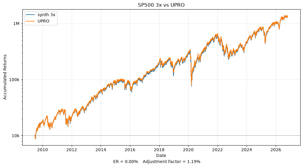
The cost of UPRO is 1.19% p.a. higher than expected
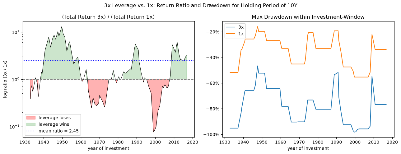
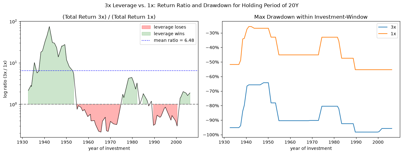
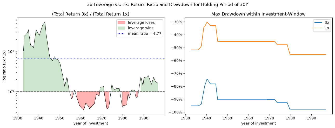
A drawdown of ~90% is realized on long holding periods
1. Import Data
2. Calculate Leveraged Daily Returns
2.1 Calculate Daily Returns $r_{basis}(t)$
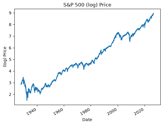
To ease the calculation, we fill every date for which no price is given with the last available price.
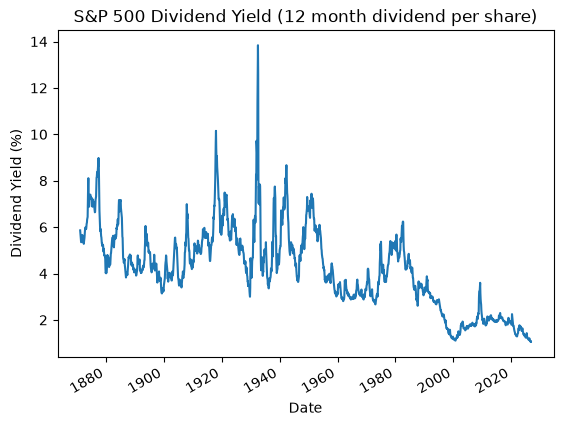
In practice dividends are paid as a lump sum at the end of each month. In order to calculate daily returns, we assume that the monthly dividend $y_m$ is paid daily and is equally distributed.
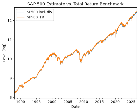
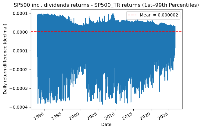
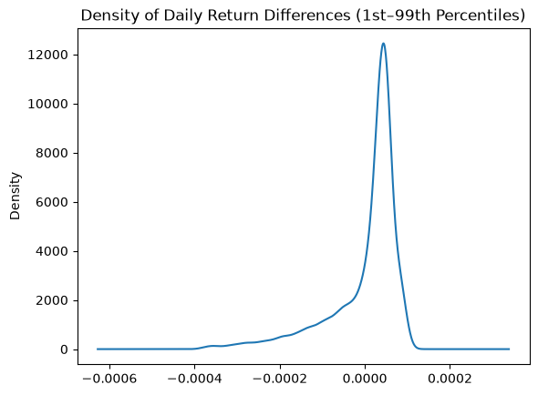
$$ y(t) = \left(1 + y_m\right)^{\frac{1}{365}} - 1 \text{ for all } t\in m$$Daily returns are the sum of daily price returns and daily dividend returns. We test the results against the S&P 500 Total Return benchmark. The residuals between the 1st and 99th quantile are low. The density of return deltas forms a left tail, since the benchmark books a whole chunk of dividends at once.
$$ r_{basis}(t) = \frac{P(t)}{P(t-1)}-1 + \frac{y(t)}{365}$$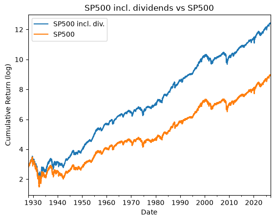
2.2 Calculate Leveraged Daily Returns
Sounds easy in theory. Calculate the daily profits of the underlying and multiply with the leverage. Subtract the cost for the ETF (Expense Ratio ER(t)) and the cost of borrowing money for the leverage (Borrowing Cost BC(t)). Also subtract a daily Adjustment Error A(t). We will set the adjustment error to 1.19% p.a. for all t as calculated in Section 2.4.
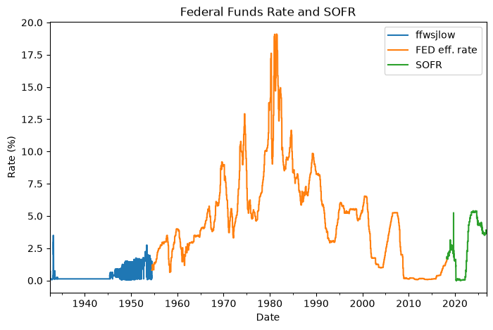
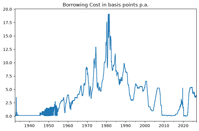
$$r_{LETF}(t) = L \cdot r_{basis}(t) - ER(t) - (L-1)\cdot BC(t) - A(t)$$The cost of borrowing money is given by the overnight borrowing rate. We use the FED interest rate starting from 1955 as a proxy for the overnight borrowing rate until SOFR was introduced in 2018. For 1932 to 1955 we use the Low Value of the Federal Funds Rate for the Indicated Date Published in The Wall Street Journal, even though this dataset is messy.
$$ BC(t) = \text{SOFR}(t)\cdot \mathbb{1}_{t > 2018} + \text{FED IR}(t)\cdot \mathbb{1}_{t <= 2018}$$The total expense ratio for the UPRO is around 0.89% p.a. (see the ProShares factsheet). In reality UPRO also pays a swap spread, which is covered by the adjustment factor below. We choose ER to be 0.89%.
$$ ER(t) = (1.0089)^\frac{1}{365} - 1$$The adjustment factor is set to 1.19% p.a. to fit the curve of the UPRO better. It seems that after 2024, the cost of the UPRO increased. Adjustment factor and expense ratio add up to about 2.08% p.a., which is higher than the anticipated 0.89%.
We calculate daily leveraged returns for all $L$ in $\{1, 1.25, ..., 3.75, 4\}$ and compare the 3x leverage with the UPRO.
2.3 Visualizing and drawdowns
In order to visualize the extreme drawdowns in the leverage, we use the maximum drawdown. Let $S_t$ be the value of cumulated returns at day $t$ and $M_t$ the maximum up to time $t$. Let $D_t$ be the percentage loss from the peak.
$$ M_t = \max_{u\leq t}S_u \ \ \ \ D_t = \frac{S_t}{M_t}-1$$We define the max drawdown as the most negative percentage loss from the last peak at time t.
$$ \text{MaxDD} = \min_t{D_t}$$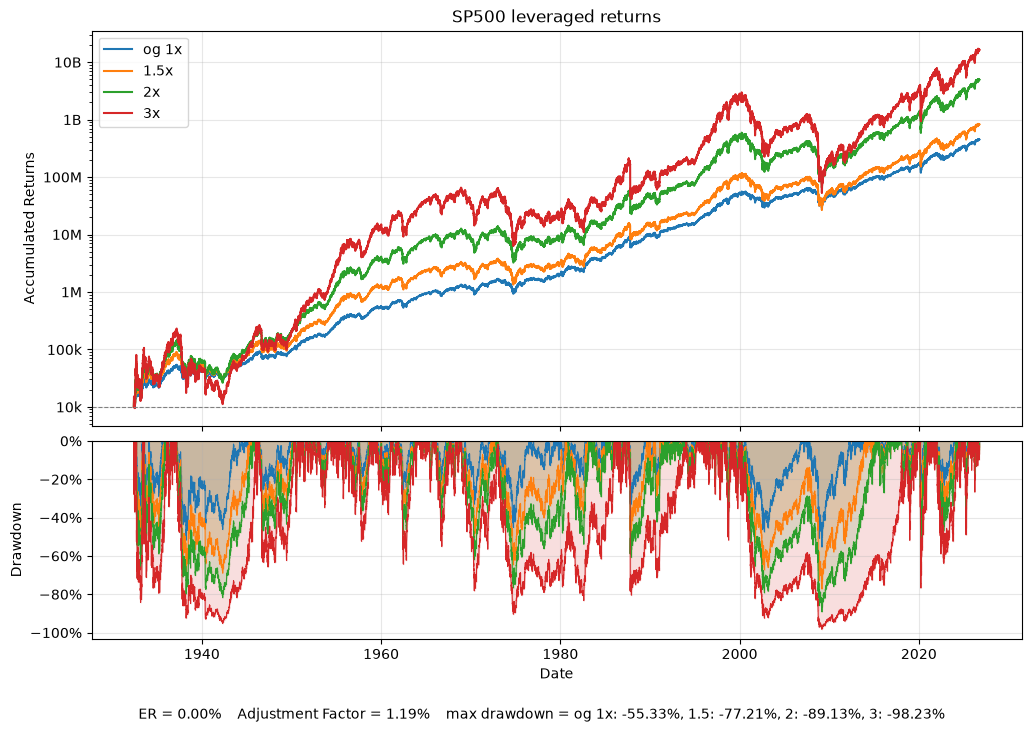
2.4 Validate 3x Leveraged Returns against UPRO
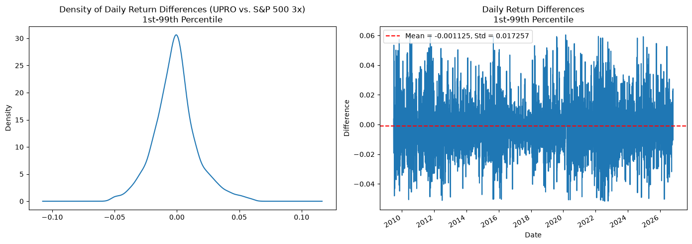
In order to check if the calculated returns are suitable, we check the 3x S&P 500 against UPRO. We have UPRO data since 2008. We set the adjustment factor to be the average difference between synthetic 3x returns (with adjustment factor 0) and UPRO returns.
2.4.1 Approximate adjustment factor
The constant annual adjustment $a^*$ is found numerically by minimising the sum of squared differences between the synthetic 3x wealth path $S_t(a)$ and the UPRO path $S^{\text{UPRO}}_t$, i.e.
$$a^* = \arg\min_a \sum_t \big(S_t(a) - S^{\text{UPRO}}_t\big)^2$$The optimization yields an optimal annual adjustment of 1.1911%.
2.4.2 Compare synthetic 3x vs UPRO
3. Result Analysis
3.1 Single investment for different holding periods
Assume that for every year in the period (1952-2026) two equally big investments in the 3x S&P 500 and the non-leveraged S&P 500 are taken on a random day $t=0$ in that year. Assume further that this investment is held for $H\in \{1,10,20,30\}$ years. Compare the returns of the investments by dividing leveraged returns by non-leveraged returns. Let $P(t)$ be the cumulated percentage return of the investments. Also compare the max drawdown of the investments in that timeframe.
$$ r_{\text{total}} = \frac{P(H)}{P(0)}, \ \ \ \ r_{\text{ratio}}=\frac{r_{\text{total 3x}}}{r_{\text{total 1x}}}$$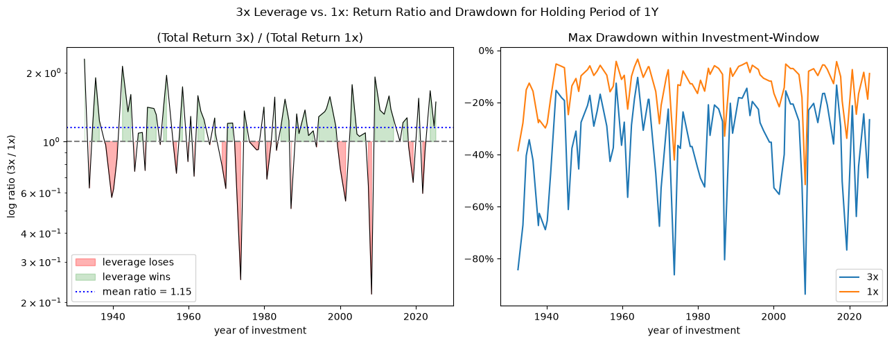
3.2 Invest every month
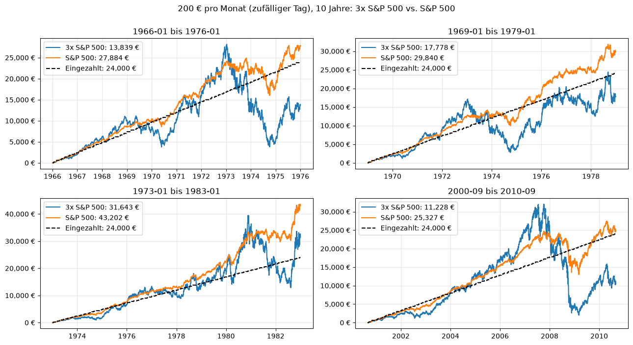
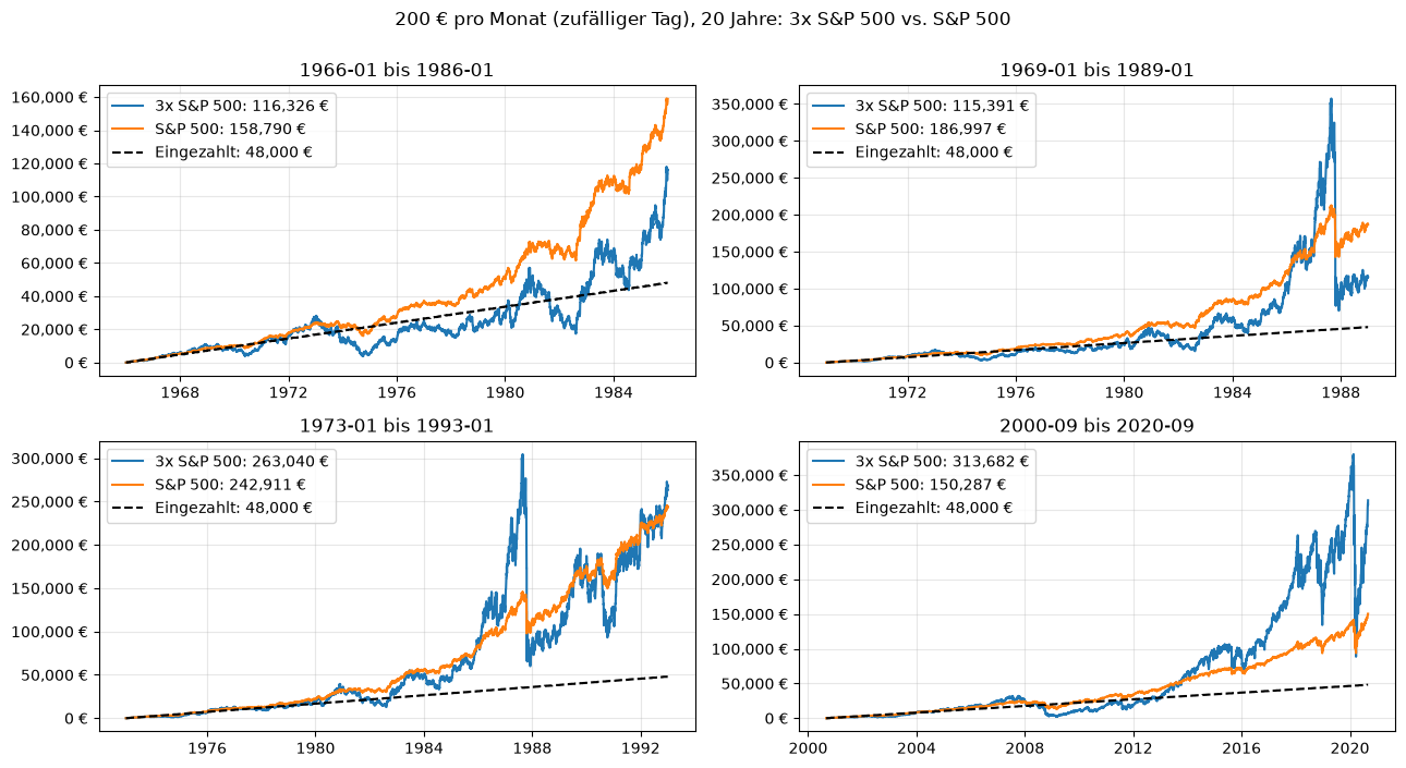
Assume that 200€ are invested on a random day in a month for 10 years or 20 years in the 3x S&P 500 and the S&P 500. As a starting period, choose the following dates:
| Start | Window | Why it was tough |
|---|---|---|
| 1966-01 | 1966–1976 | Start near the 1966 peak. Nominal index went sideways for years, with several bear markets (1966, 1968–70, 1973–74). Inflation and interest rates kept rising, so borrowing costs ate the leverage. |
| 1969-01 | 1969–1979 | Start just after the 1968 peak. Bear market 1969–70, then the 1973–74 crash (about -48%), followed by stagflation. Weak real returns and high rates. |
| 1973-01 | 1973–1983 | Start right at the top before the 1973–74 crash (about -48%), then oil shocks and Volcker-era rates (Fed funds near 19% in 1981). The worst case for a leveraged strategy. |
| 2000-09 | 2000–2010 | Start near the dotcom peak. Two bear markets (2000–02 and 2007–09, each around -50%) and a 10-year return close to zero (“lost decade”). |
Monthly investments over 10 years:
Monthly investments over 20 years:
4. 3x 30Y Treasury ETF
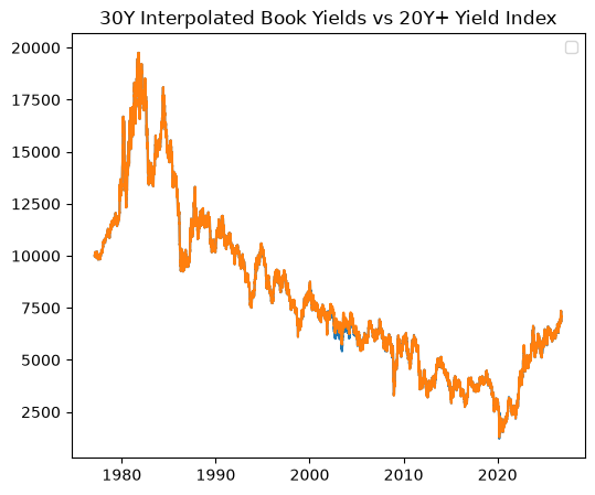
A young retail investor suggested in 2019 to hedge the huge downside risk of 3x S&P 500 with 3x leverage on the 30Y Treasury Yield fund TYX (the post is linked in [6]). This fund was set up in 1985 [7]. Data for Market Yield on U.S. Treasury Securities at 30-Year Constant Maturity at the FED starts in 1977 ([8]). A user in the blog noted above fortunately typed monthly treasury yields starting from 1941, given in a book, into a spreadsheet ([9]).
We interpolate data from 1941 until 1977 from monthly to daily by linear interpolation.
$$ y(t) = y(t_0) + \frac{t-t_0}{t_1-t_0}\left(y(t_1)-y(t_0)\right), \ \ \ \text{for all }t\in (t_0,t_1) $$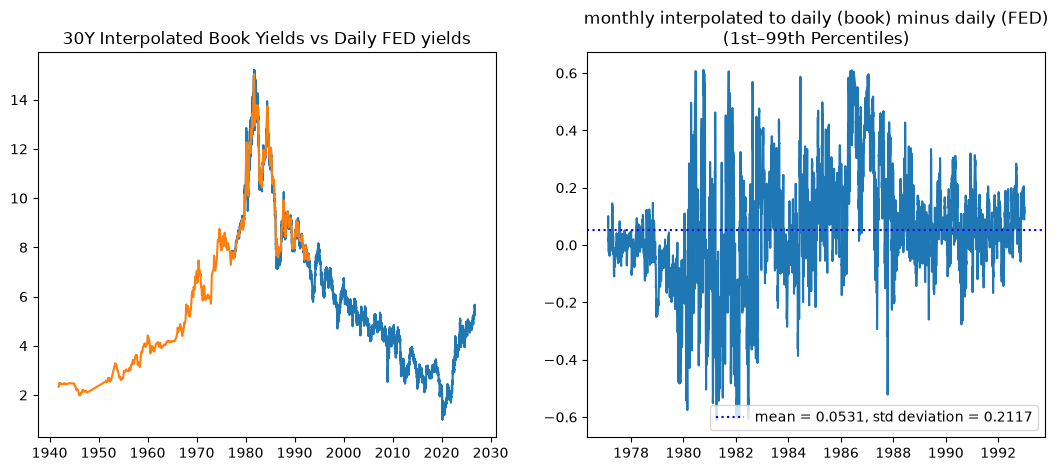
To be continued
The next goal is to derive returns of treasury funds using the yield curve.